


本文转载自微信公众号「区块链研究实验室」,作者链三丰。转载本文请联系区块链研究实验室公众号。
在本文中,我们将讨论与比特币价格预测有关的程序。
In this paper, we will discuss procedures relating to price forecasts for bitcoin.
涉及的主题:
Topics covered:
1.什么是比特币
What's Bitcoin?
2.如何使用比特币
2. How to use Bitcoin
3.使用深度学习预测比特币价格
3. Use of in-depth learning to predict bitcoin prices
比特币是所有加密爱好者普遍使用的加密货币之一。即使有几种突出的加密货币,如以太坊,Ripple,Litecoin等,比特币也位居榜首。
Bitcoin is one of the encrypted currencies commonly used by encryption fans. Bitcoin is at the top of the list even if there are several prominent encrypt currencies, such as Etheria, Ripple, Litecoin, etc.
加密货币通常用作我们货币的加密形式,广泛用于购物,交易,投资等。
Encrypted money is usually used as a form of encryption for our money, and is widely used for shopping, transactions, investments, etc.
它使用对等技术,该技术背后是,没有驱动力或任何第三方来干扰网络内完成的交易。此外,比特币是“开源的”,任何人都可以使用。
It uses the technology of reciprocity, behind which there is no drive or any third party to interfere with transactions done within the network. Besides, Bitcoin is &ldquao; open source & rdquao; anyone can use it.
功能:
- 快速的点对点交易
- 全球支付
- 手续费低
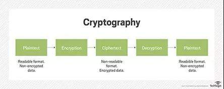
使用的原理-密码学:
Rationale for use by
加密货币(比特币)背后的工作原理是“加密”,他们使用此原理来保护和认证协商,并控制加密货币新组件的建立。
The working principles behind the encrypt currency (bitcoin) are “ encrypt & rdquao; they use this to protect and authenticate consultations and control the creation of new components of the encrypt currency.
- 保护钱包:应该更安全地保护比特币钱包,以便轻松顺利地进行交易
- 比特币价格易变:比特币价格可能会波动。价格可以根据通货膨胀率,数量等几个因素而增加或减少。

1. 数据收集:
Data collection:
导入CSV文件数据集。
Imports the CSV file data set.
- import pandas as pd
- import numpy as np
- import matplotlib.pyplot as plt
现在,使用pandas和numpy导入数据集。Numpy主要用于python中的科学计算,
Now, the data sets are imported using pandas and numpy. Numpy is used mainly for scientific calculations in python.
- coindata = pd.read_csv(‘Dataset.csv’)
- googledata = pd.read_csv(‘DS2.csv’)
已加载的原始数据集已打印,
The original data set that has been loaded has been printed.
- coindata = coindata.drop([‘#’], axis=1)
- coindata.columns = [‘Date’,’Open’,’High’,’Low’,’Close’,’Volume’]
- googledata = googledata.drop([‘Date’,’#’], axis=1)
未使用的列将放在此处。
Unused columns will be placed here.
从硬币数据和Google数据集中删除两列,因为它们是未使用的列。
Two columns were removed from the coin data and the Google data set because they were unused columns.
从数据集中删除未使用的列后,将为两个数据集打印最终结果。
After removing the unused columns from the data set, the final results will be printed for both data sets.
- last = pd.concat([coindata,googledata], axis=1)
将两个数据集(硬币数据和谷歌数据)连接起来,并使用函数将其打印出来
Connect two data sets (coins and Google data) and print them out using a function
- last.to_csv(‘Bitcoin3D.csv’, index=False)
2.一维RNN:
2. One-dimensional RNN:
现在将两个数据集串联后,将导出最终数据集。
The two data sets are now linked and the final data sets will be exported.
- import pandas as pd
- import matplotlib.pyplot as plt
- import numpy as np
- import math
- from sklearn.preprocessing import MinMaxScaler
- from sklearn.metrics import mean_squared_error
- from keras.models import Sequential
- from keras.layers import Dense, Activation, Dropout
- from keras.layers import LSTM
在这里使用Keras库。Keras仅需几行代码即可使用有效的计算库训练神经网络模型。
This is where Keras library is used. Keras uses only a few lines of code to train neural network models using an effective calculator.
MinMaxScaler会通过将每个特征映射到给定范围来转换特征。sklearn软件包将提供该程序所需的一些实用程序功能。
MinMaxScaler converts features by mapping each feature to a given range.
密集层将执行以下操作,并将返回输出。
The dense layer will perform the following operations and will return the output.
- output = activation(dot(input, kernel) + bias)
- def new_dataset(dataset, step_size):
- data_X, data_Y = [], []
- for i in range(len(dataset)-step_size-1):
- a = dataset[i:(i+step_size), 0]
- data_X.append(a)
- data_Y.append(dataset[i + step_size, 0])
- return np.array(data_X), np.array(data_Y)
将在数据预处理阶段收集的一维数据分解为时间序列数据,
Disassemble one dimension of the data collected during the pre-processing phase into time-series data,
- df = pd.read_csv(“Bitcoin1D.csv”)
- df[‘Date’] = pd.to_datetime(df[‘Date’])
- df = df.reindex(index= df.index[::-1])
数据集已加载。该功能是从Bitcoin1D.csv文件中读取的。另外,将“日期”列转换为“日期时间”。通过“日期”列重新索引所有数据集。
The data set is loaded. This function is read from the Bitcoin1D.csv file. Also, converts &ldquao; date&rdquao; column to &ldquao; date time & rdquao; & by &ldquao; date & & rdquao; column reindexing all data sets.
- zaman = np.arange(1, len(df) + 1, 1)
- OHCL_avg = df.mean(axis=1)
直接分配一个新的索引数组。
Directly assigns a new index array.
- OHCL_avg = np.reshape(OHCL_avg.values, (len(OHCL_avg),1)) #7288 data
- scaler = MinMaxScaler(feature_range=(0,1))
- OHCL_avg = scaler.fit_transform(OHCL_avg)
分配定标器后规格化数据集,
To assign a standardised data set after the marker,
- #print(OHCL_avg)
- train_OHLC = int(len(OHCL_avg)*0.56)
- test_OHLC = len(OHCL_avg) — train_OHLC
- train_OHLC, test_OHLC = OHCL_avg[0:train_OHLC,:], OHCL_avg[train_OHLC:len(OHCL_avg),:]
- #Train the datasets and test it
- trainX, trainY = new_dataset(train_OHLC,1)
- testX, testY = new_dataset(test_OHLC,1)
从平均OHLC(开高低开)中创建一维维度数据集,
To create a one-dimensional data set from the average OHLC (high and low)
- trainX = np.reshape(trainX, (trainX.shape[0],1,trainX.shape[1]))
- testX = np.reshape(testX, (testX.shape[0],1,testX.shape[1]))
- step_size = 1
以3D维度重塑LSTM的数据集。将step_size分配给1。
Recreates the LSTM data set in 3D dimensions. Step_size is assigned to 1.
- model = Sequential()
- model.add(LSTM(128, input_shape=(1, step_size)))
- model.add(Dropout(0.1))
- model.add(Dense(1))
- model.add(Activation(‘linear’))
创建LSTM模型,
Create an LSTM model,
- model.compile(loss=’mean_squared_error’, optimizer=’adam’)
- model.fit(trainX, trainY, epochs=10, batch_size=25, verbose=2)
将纪元数定义为10,batch_size为25,
Defines the number of periods as 10, batts_size to 25,
- trainPredict = model.predict(trainX)
- testPredict = model.predict(testX)
- trainPredict = scaler.inverse_transform(trainPredict)
- trainY = scaler.inverse_transform([trainY])
- testPredict = scaler.inverse_transform(testPredict)
- testY = scaler.inverse_transform([testY])
完成了归一化以进行绘图,
It's done. It's done. It's done.
- trainScore = math.sqrt(mean_squared_error(trainY[0],
- trainPredict[:,0]))
- testScore = math.sqrt(mean_squared_error(testY[0],
- testPredict[:,0]))
针对预测的测试数据集计算性能度量RMSE,
RMSE for the projected test data set,
- trainPredictPlot = np.empty_like(OHCL_avg)
- trainPredictPlot[:,:] = np.nan
- trainPredictPlot[step_size:len(trainPredict)+step_size,:] =
- trainPredict
将转换后的train数据集用于绘图,
To use the converted Train data set for mapping,
- testPredictPlot = np.empty_like(OHCL_avg)
- testPredictPlot[:,:] = np.nan
- testPredictPlot[len(trainPredict)+(step_size*2)+1:len(OHCL_avg)-1,:]
- = testPredict
将转换后的预测测试数据集用于绘图,
To use the converted prognosis test data set for mapping,
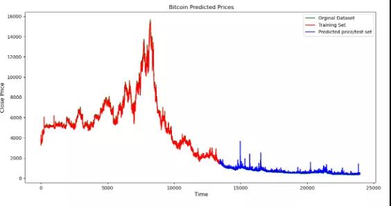
最终将预测值可视化。
Eventually, the forecast is visualized.
- OHCL_avg = scaler.inverse_transform(OHCL_avg)
- plt.plot(OHCL_avg, ‘g’, label=’Orginal Dataset’)
- plt.plot(trainPredictPlot, ‘r’, label=’Training Set’)
- plt.plot(testPredictPlot, ‘b’, label=’Predicted price/test set’)
- plt.title(“ Bitcoin Predicted Prices”)
- plt.xlabel(‘ Time’, fontsize=12)
- plt.ylabel(‘Close Price’, fontsize=12)
- plt.legend(loc=’upper right’)
- plt.show()
3.多变量的RNN:
3. Multivariant RNN:
- import pandas as pd
- from pandas import DataFrame
- from pandas import concat
- from math import sqrt
- from numpy import concatenate
- import matplotlib.pyplot as pyplot
- import numpy as np
- from sklearn.metrics import mean_squared_error
- from sklearn.preprocessing import MinMaxScaler
- from keras import Sequential
- from keras.layers import LSTM, Dense, Dropout, Activation
- from pandas import read_csv
使用Keras库。Keras仅需几行代码就可以使用有效的计算库来训练神经网络模型。sklearn软件包将提供该程序所需的一些实用程序功能。
The Keras library is used. Keras only needs a few lines of code to use an effective computing library to train a neuronetwork model. The Sklearn package will provide some of the practical program functions required for the program.
密集层将执行以下操作,并将返回输出。
The dense layer will perform the following operations and will return the output.
- dataset = read_csv(‘Bitcoin3D.csv’, header=0, index_col=0)
- print(dataset.head())
- values = dataset.values
使用Pandas库加载数据集。在这里准备了可视化的列。
Loads data sets using the Pandas library. A visual column is prepared here.
- groups = [0, 1, 2, 3, 5, 6,7,8,9]
- i = 1
将系列转换为监督学习。
Converts the series to supervisory learning.
- def series_to_supervised(data, n_in=1, n_out=1, dropnan=True):
- n_vars = 1 if type(data) is list else data.shape[1]
- df = DataFrame(data)
- cols, names = list(), list()
- # Here is created input columns which are (t-n, … t-1)
- for i in range(n_in, 0, -1):
- cols.append(df.shift(i))
- names += [(‘var%d(t-%d)’ % (j+1, i)) for j in range(n_vars)]
- #Here, we had created output/forecast column which are (t, t+1, … t+n)
- for i in range(0, n_out):
- cols.append(df.shift(-i))
- if i == 0:
- names += [(‘var%d(t)’ % (j+1)) for j in range(n_vars)]
- else:
- names += [(‘var%d(t+%d)’ % (j+1, i)) for j in
- range(n_vars)]
- agg = concat(cols, axis=1)
- agg.columns = names
- # drop rows with NaN values
- if dropnan:
- agg.dropna(inplace=True)
- return agg
检查值是否为数字格式,
Check if the value is in numerical format,
- values = values.astype(‘float32’)
数据集值通过使用MinMax方法进行归一化,
Dataset values are being normalized using the MinMax method.
- scaler = MinMaxScaler(feature_range=(0,1))
- scaled = scaler.fit_transform(values)
将规范化的值转换为监督学习,
To convert the normative values into supervisory learning,
- reframed = series_to_supervised(scaled,1,1)
- #reframed.drop(reframed.columns[[9,10,11,12,13,14,15]], axis=1, inplace=True)
数据集分为两组,分别是训练集和测试集,
The data sets are divided into two groups: a training set and a test set.
- values = reframed.values
- train_size = int(len(values)*0.70)
- train = values[:train_size,:]
- test = values[train_size:,:]
拆分的数据集被拆分为trainX,trainY,testX和testY,
Disaggregated data sets are divided into trainX, trainY, testX and testy,
- trainX, trainY = train[:,:-1], train[:,13]
- testX, testY = test[:,:-1], test[:,13]
训练和测试数据集以3D尺寸重塑以用于LSTM,
Training and testing of data sets for remodelling at 3D dimensions for use in LSTM.
- trainX = trainX.reshape((trainX.shape[0],1,trainX.shape[1]))
- testX = testX.reshape((testX.shape[0],1,testX.shape[1]))
创建LSTM模型并调整神经元结构,
Creates an LSTM model and adjusts the neuron structure.
- model = Sequential()
- model.add(LSTM(128, input_shape=(trainX.shape[1], trainX.shape[2])))
- model.add(Dropout(0.05))
- model.add(Dense(1))
- model.add(Activation(‘linear’))
- model.compile(loss=’mae’, optimizer=’adam’)
通过使用trainX和trainY训练数据集,
Through the use of trainX and trainY training data sets,
- history = model.fit(trainX, trainY, epochs=10, batch_size=25, validation_data=(testX, testY), verbose=2, shuffle=False)
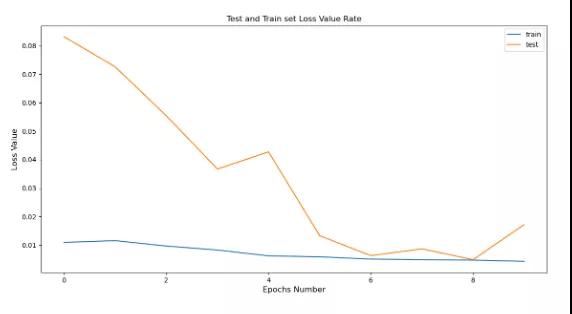
计算每个训练时期的损耗值,并将其可视化,
Calculate and visualize the loss values of each training period,
- pyplot.plot(history.history[‘loss’], label=’train’)
- pyplot.plot(history.history[‘val_loss’], label=’test’)
- pyplot.title(“Test and Train set Loss Value Rate”)
- pyplot.xlabel(‘Epochs Number’, fontsize=12)
- pyplot.ylabel(‘Loss Value’, fontsize=12)
- pyplot.legend()
- pyplot.show()
对训练数据集执行预测过程,
Implementing a forecasting process for training data sets,
- trainPredict = model.predict(trainX)
- trainX = trainX.reshape((trainX.shape[0], trainX.shape[2]))
对测试数据集执行预测过程,
Implementing a forecasting process for test data sets,
- testPredict = model.predict(testX)
- testX = testX.reshape((testX.shape[0], testX.shape[2]))
训练数据集反转缩放比例以进行训练,
Training in reverse scaling of data sets for training,
- testPredict = model.predict(testX)
- testX = testX.reshape((testX.shape[0], testX.shape[2]))
测试数据集反转缩放以进行预测,
Test datasets for inverting to make predictions,
- testPredict = concatenate((testPredict, testX[:, -9:]), axis=1)
- testPredict = scaler.inverse_transform(testPredict)
- testPredict = testPredict[:,0]
- # invert scaling for actual
- testY = testY.reshape((len(testY), 1))
- inv_y = concatenate((testY, testX[:, -9:]), axis=1)
- inv_y = scaler.inverse_transform(inv_y)
- inv_y = inv_y[:,0]
通过将mean_squared_error用于train和测试预测来计算性能指标,
To calculate performance indicators by using mean_squared_error for train and testing predictions,
- rmse2 = sqrt(mean_squared_error(trainY, trainPredict))
- rmse = sqrt(mean_squared_error(inv_y, testPredict))
训练和测试的预测集串联在一起
The sequence of predictions of training and testing is linked together.
- final = np.append(trainPredict, testPredict)
- final = pd.DataFrame(data=final, columns=[‘Close’])
- actual = dataset.Close
- actual = actual.values
- actual = pd.DataFrame(data=actual, columns=[‘Close’])
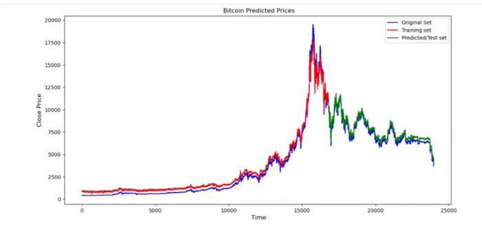
最后,将训练和预测结果可视化。
Finally, the results of training and forecasting will be visualized.
- pyplot.plot(actual.Close, ‘b’, label=’Original Set’)
- pyplot.plot(final.Close[0:16781], ‘r’ , label=’Training set’)
- pyplot.plot(final.Close[16781:len(final)], ‘g’,
- label=’Predicted/Test set’)
- pyplot.title(“ Bitcoin Predicted Prices”)
- pyplot.xlabel(‘ Time’, fontsize=12)
- pyplot.ylabel(‘Close Price’, fontsize=12)
- pyplot.legend(loc=’best’)
- pyplot.show()
目前为止,我们使用历史比特币价格数据集开发价格预测模型,通过使用Python中的RNN和LSTM算法来找到价格预测。
So far, price forecasting models have been developed using historical bitcoin price data sets, and price forecasts have been found using RNN and LSTM algorithms in Python.
注册有任何问题请添加 微信:MVIP619 拉你进入群

打开微信扫一扫
添加客服
进入交流群


发表评论